.png)

Motion Problems – A Glimpse into Calculus
- Juliana Luan
- May 8, 2024
- 2 min read
What is your first impression of calculus? Advanced, intimidating, or intriguing? Students often perceive calculus as an abstruse and topic which requires significant effort to understand, but this is not the case.
Calculus is a mathematical way of thinking that simplifies complex problems through the transformation of dimensions. It can be applied to calculate volumes and areas, to determine the rate of change at any moment, and to achieve many other incredible things. Today we will be discussing its application in motion problems, a classic topic in Newtonian physics.
Equations of Motion
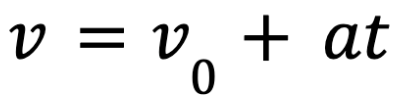
Most of us have gone through the calculation of acceleration, velocity and displacement, and we must be familiar with the following equations of motion:
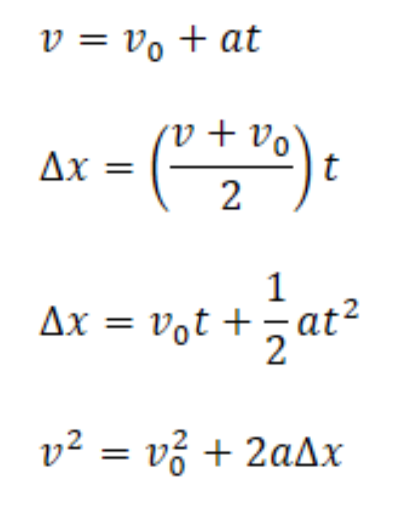
But have you ever wondered about the origins of these equations? How was the third equation found? Here is a simple calculus proof.
In the proof we introduce Riemann sum, which is an approximation of the area under a function obtained by summing areas of infinite small areas (rectangles). The three graphs below show the same function f(x), the velocity of a particle, over a time period (a to b). To calculate the displacement over a time period, we can split x-axis (time) into smaller parts. Each part is a thin rectangle, as shown in the first graph. We know s = vt, so the displacement during that tiny time slot can be referred to the area of the small rectangle, whose length is v and width is t.
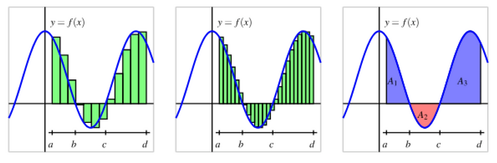
By adding the area of these tiny rectangle together, we have the total displacement over t. You may say this approximation isn’t accurate, because some rectangles may overestimate or underestimate the displacement over that time period, given that the velocity function is not a horizontal line. But if we make the width infinitely small, the approximation will get more precise, and eventually the overestimation/underestimation can be ignored, as shown in the second graph.
This is where calculus is applied, more specifically, integrals. We can make something infinitely small to eliminate the error, therefore creating another formula to describe the cumulative sum of the first function. The formula can be expressed as:

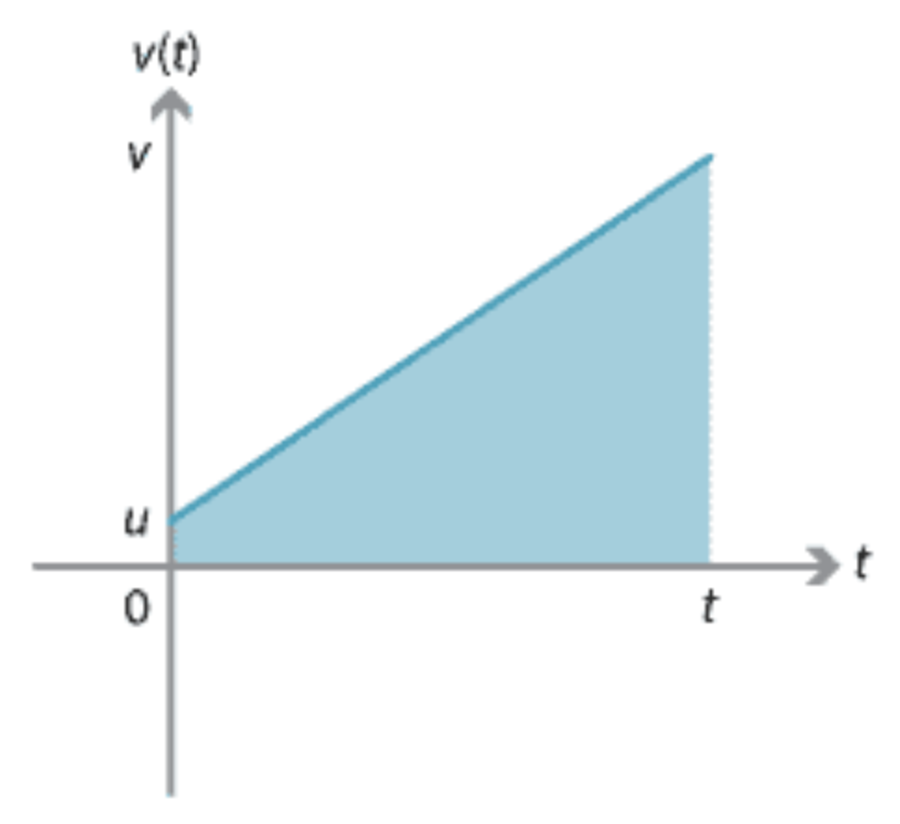
Therefore, the total displacement is the area under the function curve. If the acceleration is constant, the area would look like a trapezoid (see the graph below).
Given the function of trapezoid area:
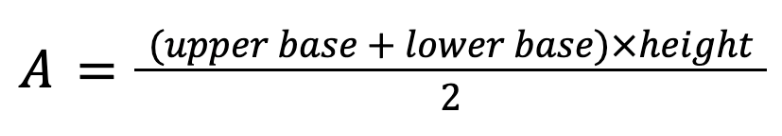
We have:
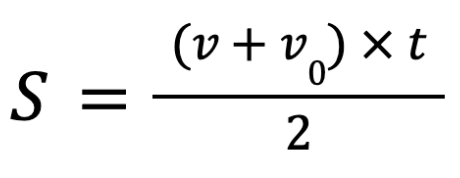
Since

And here we have the second formula of motion problems!
If you are interested in exploring the power of calculus after going through the proof above, I highly encourage you to read more material on Khan Academy AP Calculus BC, which I use as a self-learning tool. Rather than mindlessly memorizing equations, you can fully grasp how these equations are derived, and will be fascinated by its rigorous logic and unparalleled imagination.
Work Cited
Activecalculus.org. (2024). AC Riemann Sums. [online] Available at: https://activecalculus.org/single/sec-4-2-Riemann.html [Accessed 8 Apr. 2024].
Amsi.org.au. (2024). Content - Constant acceleration. [online] Available at: https://amsi.org.au/ESA_Senior_Years/SeniorTopic3/3i/3i_2content_3.html [Accessed 8 Apr. 2024].
Brilliant.org. (2024). Riemann Sums | Brilliant Math & Science Wiki. [online] Available at: https://brilliant.org/wiki/riemann-sums. [Accessed 8 Apr. 2024].
Khanacademy.org. (2023). Khan Academy. [online] Available at: https://www.khanacademy.org/math/ap-calculus-bc [Accessed 8 Apr. 2024].
MechanicallyChallenged (2023). speed acceleration stretch formulas physics | Medium. [online] Medium. Available at: https://medium.com/@MechanicallyChallenged/the-four-basic-equations-in-kinematics-6463a146af9 [Accessed 8 Apr. 2024].
Commentaires